Computer Vision: Non-Linear Optimization Methods

This is a brief summary of some of the optimization methods used in Computer Vision topics like Camera Calibration and 3D-Reconstructions.

---

We’re going to start with a relatively simple method and work our way to the more complicated but also a lot more powerful method that’s actually used in computer vision topics.

Newton’s Method

The simplest method we can use is Newton’s method. We first look at it in 1 dimension, then in higher dimensions and finally we consider some extensions.

Newton’s Method in 1D

Given a function

$$f: \mathbb{R} \rightarrow \mathbb{R}$$

find

$$\min_{x \in \mathbb{R}} f(x).$$

To solve this problem we look for the offset $dx$ that minimizes $f(x + dx)$. We start by writing the Taylor expansion of $f(x + dx)$,

$$f(x + dx) = f(x) + f'(x) dx + \frac{1}{2} f”(x) dx^2 + O(dx^3).$$

The Taylor expansion can be written with (infinitely) many terms but in Newton’s method we only keep the first three terms (and we assume the others are negligible). To minimize this function we first take its derivative,

$$\frac{d}{dx} f(x + dx) = f'(x) + f”(x) dx$$

and set it to zero

$$f'(x) + f”(x) dx = 0.$$

Solving for $dx$ gives

$$ dx = – \frac{f'(x)}{f”(x)}.$$

By moving $x$ in the direction of $dx$ we change the function value. If $f”(x)$ is positive then $f(x + dx) < f(x)$ (unless we overshoot), if it’s negative then $f(x + dx) > f(x)$ and if it’s zero then we’re in a locally linear section of $f$ and we can’t actually compute $dx$. So for a minimization method we ideally want to have $f”(x) > 0$¹.

After we’ve computed $dx$ we evaluate $f$ at $x + dx$, but we’re most probably not at the minimum of $f$. And that’s because we used the information $f'(x)$ and $f”(x)$ at point $x$ to compute the offset. But the function value changes as soon as we move away from $x$ and thus the first and second derivatives at $x$ will no longer be accurate. So what we computed above is really just an estimate. To find a minimum we have to repeat the same process again, so we start at some estimate $x_0$ and we compute

$$x_{k+1} = x_{k}\ -\ \frac{f'(x_k)}{f”(x_k)}$$

until

$$\left| \frac{f'(x_k)}{f”(x_k)} \right| \approx 0.$$

Following this recipe allows us to find a local optimum (unless we get stuck in a locally linear section). There is no guarantee that we’ll find the global optimum.

Newton’s Method in ND

In higher dimensions we have

$$f: \mathbb{R}^N \rightarrow \mathbb{R}.$$

The first derivative is replaced by the gradient and the second by the Hessian matrix,

$$
\nabla f =
\begin{bmatrix}
\frac{\partial f}{\partial x_1} \\
\frac{\partial f}{\partial x_2} \\
\vdots \\
\frac{\partial f}{\partial x_N}
\end{bmatrix},
\quad
\nabla^2 f =
\begin{bmatrix}
\frac{\partial^2 f}{\partial x_1^2} & \frac{\partial^2 f}{\partial x_1 \partial x_2} & \cdots & \frac{\partial^2 f}{\partial x_1 \partial x_N} \\
\frac{\partial^2 f}{\partial x_2 \partial x_1} & \frac{\partial^2 f}{\partial x_2^2} & \cdots & \frac{\partial^2 f}{\partial x_2 \partial x_N} \\
\vdots & \vdots & \ddots & \vdots \\
\frac{\partial^2 f}{\partial x_N \partial x_1} & \frac{\partial^2 f}{\partial x_N \partial x_2} & \cdots & \frac{\partial^2 f}{\partial x_N^2}
\end{bmatrix}.
$$

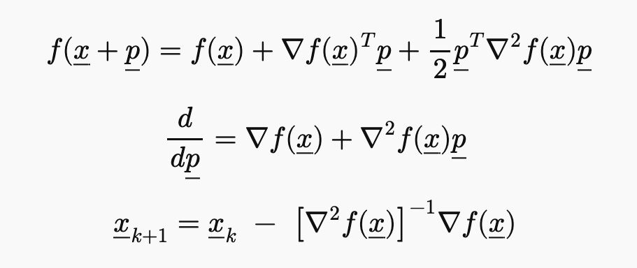
The Taylor expansion becomes

$$f(\underline{x} + \underline{p}) = f(\underline{x}) + \nabla f(\underline{x})^T \underline{p} + \frac{1}{2} \underline{p}^T \nabla^2 f(\underline{x}) \underline{p}$$

and its derivative becomes

$$\frac{d}{d\underline{p}} = \nabla f(\underline{x})+ \nabla^2 f(\underline{x}) \underline{p}.$$

Setting it to zero and solving for $\underline{p}$ gives

$$\underline{x}_{k+1} = \underline{x}_k\ -\ \left[ \nabla^2 f(\underline{x}) \right]^{-1} \nabla f(\underline{x}).$$

This requires us to compute the Hessian matrix (and it must be invertible). To guarantee convergence to a local minimum the Hessian also needs to be positive-definite (i.e. all eigenvalues must be positive). If the Hessian is indefinite then we may converge to a saddle point or if it’s negative-definite then we may converge to a maximum. If it’s positive-definite but the eigenvalues are small then we may get huge or unstable steps.

Extensions

There are a few extensions to Newton’s method that make it more stable. I’m just putting them here so I can remember them, feel free to skip to the next method.

Line Search

Rather than taking a full step

$$\underline{x}_{k+1} = \underline{x}_k + \underline{p}_k$$

where

$$ \underline{p}_k = – \left[ \nabla^2 f(\underline{x}) \right]^{-1} \nabla f(\underline{x})$$

we adjust the equation to

$$\underline{x}_{k+1} = \underline{x}_k + \lambda \underline{p}_k \text{ for some } \lambda \in \mathbb{R}.$$

Our objective is to find a $\lambda$ that prevents us from overshooting but that also doesn’t stall (become too small).

There are different ways to find $\lambda$. A simple way is to start with $\lambda = 1$ and to check if the Armijo (and Wolfe) conditions are satisfied.

$\lambda$ can be reduced by multiplying it by some $\beta \in (0, 1)$. Armijo may lead to very small steps. This can be prevented by using Wolfe’s condition. However, that would require a more complicated algorithm, which I won’t cover here.

Trust-Region

We approximate $f$ locally with a quadratic model

$$ m_k(\underline{p}) = f(\underline{x}_k) + \left[\nabla f(\underline{x}_k) \right]^T \underline{p} + \frac{1}{2} \underline{p}^T \nabla^2 f(\underline{x}_k) \underline{p}.$$

Now we minimize

$$ \min_{\underline{p}} m_k(\underline{p}), \quad \text{ subject to } \Vert \underline{p} \Vert \leq \Delta$$

where $\Delta$ is the trust-region radius. The update step $\underline{p}_k$ is computed as before. If $\Vert \underline{p}_k \Vert \leq \Delta_k$ then we take a full Newton step $\underline{x}_{k+1} = \underline{x}_k + \underline{p}_k$. Otherwise the solution would be outside of the trust region. In that case we use an optimization method (e.g. dogleg) to find the point on the boundary of the trust region that minimizes $m_k(\underline{p})$.

Now we’ve got a candidate $\underline{x}_{k+1}$ and we want to check if our quadratic model at $\underline{x}_{k+1}$ is reliable. So we compute the predicted decrease of the function value $m_k(\underline{0})\ -\ m_k(\underline{p}_k)$ and the actual decrease $f(\underline{x}_k)\ -\ f(\underline{x}_k + \underline{p}_k)$. If they are sufficiently similar then we trust the model, take the step, and increase $\Delta$. Otherwise we don’t trust the model, reject the step and decrease $\Delta$,

$$
\small
\rho_k =
\frac{m_k(\underline{0})\ -\ m_k(\underline{p}_k)}
{f(\underline{x}_k)\ -\ f(\underline{x}_k + \underline{p}_k)},
\quad
\text{e.g.} \quad
\left\{
\begin{aligned}
\rho_k &< \tfrac{1}{4}
&&\Rightarrow\ \text{reject},\
\underline{x}_{k+1} = \underline{x}_k,\
\Delta_{k+1} = \tfrac{1}{4}\,\Delta_k, \\[6pt]
\rho_k &\ge \tfrac{1}{4}
&&\Rightarrow\ \text{accept},\
\underline{x}_{k+1} = \underline{x}_k + \underline{p}_k,\
\Delta_{k+1} = 2\,\Delta_k
\end{aligned}
\right.
$$

This check also prevents us from taking a step in the wrong direction.

Gauss-Newton Method

So far we’ve looked at $f(\underline{x})$ without assuming any special structure. In the common case of least squares problems $f(\underline{x})$ is the sum of squared residuals,

$$f( \underline{x} ) = \tfrac{1}{2} \Vert r(\underline{x}) \Vert^2 = \tfrac{1}{2} \sum_{i=1}^M r_i^2(\underline{x}), \quad \text{with } r: \mathbb{R}^N \rightarrow \mathbb{R}^M.$$

In this case we can specify the gradient,

$$
\nabla f =
\begin{bmatrix}
\frac{\partial f}{\partial x_1} \\
\frac{\partial f}{\partial x_2} \\
\vdots \\
\frac{\partial f}{\partial x_N}
\end{bmatrix}
=
\begin{bmatrix}
\frac{\partial r_1}{\partial x_1} & \frac{\partial r_2}{\partial x_1} & \cdots & \frac{\partial r_M}{\partial x_1} \\
\frac{\partial r_1}{\partial x_2} & \frac{\partial r_2}{\partial x_2} & \cdots & \frac{\partial r_M}{\partial x_2} \\
\vdots & \vdots & \ddots & \vdots \\
\frac{\partial r_1}{\partial x_N} & \frac{\partial r_2}{\partial x_N} & \cdots & \frac{\partial r_M}{\partial x_N}
\end{bmatrix}
\begin{bmatrix}
r_1(x) \\
r_2(x) \\
\vdots \\
r_M(x)
\end{bmatrix}
=
J(\underline{x})^{T} r(\underline{x})
$$

For example, the first line can be found as

$$
\begin{aligned}
\frac{\partial f(\underline{x})}{\partial x_1}
&= \frac{\partial}{\partial x_1}
\left(
\tfrac{1}{2} r_1^2(\underline{x}) +
\tfrac{1}{2} r_2^2(\underline{x}) +
\cdots +
\tfrac{1}{2} r_M^2(\underline{x})
\right) \\[8pt]
&= r_1(\underline{x}) \frac{\partial r_1}{\partial x_1}
+r_2(\underline{x}) \frac{\partial r_2}{\partial x_1}
+\cdots
+r_M(\underline{x}) \frac{\partial r_M}{\partial x_1} \\[8pt]
&=
\begin{bmatrix}
\frac{\partial r_1}{\partial x_1} &
\frac{\partial r_2}{\partial x_1} &
\cdots &
\frac{\partial r_M}{\partial x_1}
\end{bmatrix}
\begin{bmatrix}
r_1(\underline{x}) \\[4pt]
r_2(\underline{x}) \\[2pt]
\vdots \\[2pt]
r_M(\underline{x})
\end{bmatrix}
\end{aligned}.
$$

The Hessian is

$$
\begin{aligned}
\nabla^2 f(\underline{x}) &= \nabla \left( \nabla f(\underline{x}) \right) \\
&= \nabla \left( J^T(\underline{x}) r(\underline{x}) \right) \\
&= J^T(\underline{x}) \nabla r(\underline{x}) + \nabla J^T(\underline{x}) r(\underline{x}) \\
&= J^T(\underline{x}) J(\underline{x}) + \sum_{i=1}^M r_i(\underline{x}) \nabla^2 r_i(\underline{x}).
\end{aligned}
$$

If the residuals are small, i.e. if we’re close to a solution, then the last term in the Hessian is negligible and we can approximate the Hessian with

$$ \nabla^2 f(\underline{x}) \approx J^T(\underline{x}) J(\underline{x}),$$

where $J^T J$ is always positive semi-definite. The Gauss-Newton method makes this approximation. The Taylor expansion is then

$$f(\underline{x} + \underline{p}) \approx f(\underline{x}) + J^T(\underline{x}) r(\underline{x}) \cdot \underline{p} + \frac{1}{2} \underline{p}^T J^T(\underline{x}) J(\underline{x}) \underline{p}. $$

The derivative is computed as

$$ \frac{df}{d\underline{p}} \approx J^T \underline{r} + J^T J \underline{p}$$

and the update rule is given by

$$ \underline{p} = -\left( J^T(\underline{x}) J(\underline{x})\right)^{-1} J^T(\underline{x}) \underline{r}.$$

Newton vs Gauss-Newton

Let’s briefly compare how these methods differ.

Cost

Newton requires the calculation of the Hessian which is $O(mn^2)$, Gauss-Newton only needs the gradient $O(mn)$, which is usually computed anyway.

Solving

Gauss-Newton’s $J^T J p = – J^T \underline{r}$ is equivalent to $\min_{p} \Vert J\underline{p} – \underline{r}\Vert^2$, which can be solved efficiently with QR, SVD or other decompositions. Newton’s $\nabla^2 f \underline{p} = -J^T \underline{r}$ can’t be solved that way. We have to use the Cholesky decomposition if $\nabla^2f$ is semi-positive definite and the $LDL^2$ method otherwise.

Convergence

Newton is quadratic (in theory), Gauss-Newton is (super-)linear. So if Newton works then it converges more quickly (although each step requires a lot more computation).

Issues with Gauss-Newton

While Gauss-Newton is specialized for least-squares problems there are still some issues to consider:

• Gauss-Newton drops the second term of the Hessian $\sum_{i=1}^M r_i(\underline{x}) \nabla^2 r_i(\underline{x})$. If we’re not close to the solution then this term may be large, which can cause the method to diverge.
• It requires $J(\underline{x})$ to have full-rank, otherwise $J^T J$ may be singular and we won’t be able to compute the step (or steps may not be stable).
• Far from the solution we may not converge to any solution at all.

Levenberg-Marquardt

These issues are addressed in an extension of Gauss-Newton. It can be viewed in two ways, from a damping-parameter point of view and from a trust-region point of view.

Damping Parameter View

Here we adjust the Gauss-Newton update by including a damping parameter $\lambda$,

$$ \left( J^T(\underline{x}) J(\underline{x}) + \lambda \mathbf{I} \right) \underline{p} = – J^T(\underline{x}) r(\underline{x}) \quad \text{with } \lambda \geq 0.$$

If $\lambda = 0$ then we take a pure Gauss-Newton step. If $\lambda$ is large then we take a (small) step that’s similar to steepest gradient descent, $\underline{p} = – \frac{1}{\lambda} J^T \underline{r}$.

The Algorithm goes as follows:

• Compute $J(\underline{x}_k)$ and $r(\underline{x}_k)$.
• Solve the equation above for $\underline{p}$ and compute the candidate $\underline{\tilde{x}}_{k+1}= \underline{x}_k + \underline{p}$.
• Compute the actual and expected decrease in the function value and their ratio
  $$ \rho_k = \frac{f(\underline{x}_k)\ -\ f(\underline{\tilde{x}}_{k+1})}{\frac{1}{2} \Vert r(\underline{x}_k) \Vert^2\ -\ \frac{1}{2} \Vert r(\underline{x}_k) + J^T(\underline{x}) \underline{p} \Vert^2 }. $$
• If $\rho_k$ is close to 1 then accept the candidate. So $\underline{x}_{k+1} = \underline{\tilde{x}}_{k+1}$ and $\lambda_{k+1} = \beta_1 \lambda_k$ with $\beta_1 \in (0, 1)$. Otherwise reject the candidate. So $\underline{x}_{k+1} = \underline{x}_k$ and $\lambda_{k+1} = \beta_2 \lambda_k$ with $\beta_2 > 1$.

This means that far from the solution Levenberg-Marquardt (LM) is similar to gradient descent and omitting the second term of the Hessian is not a problem. Close to the solution LM is similar to Gauss-Newton so it converges relatively quickly (super-linearly). As long as $\lambda \neq 0$, $J^T J + \lambda \mathbf{I}$ is positive-definite, so the problem can be solved.

Trust-Region View

LM can also be written as

$$\min_{\underline{p}} \Vert J^T \underline{p} + \underline{r} \Vert^2 \quad \text{subject to } \Vert \underline{p} \Vert \leq \Delta.$$

However, for the time being I’ll skip this view of LM (because I don’t feel like dealing with Lagrange multipliers right now, as I’m writing this ;).

---

Footnotes:

1. It can happen that we first move towards a maximum, overshoot, and then converge to a minimum but in general if $f”(x) < 0$ then we won’t converge to a minimum. ↩︎