
Semi-Global Matching is an algorithm that’s commonly used in Stereo Vision and also in Multi-View Stereo (e.g. when doing 3D-Reconstructions). To know more about it I first read Mr Hirschmüller’s paper that introduced SGM. Then I got two Raspberry Pi Camera Modules v3 and hooked them up to a Raspberry Pi 5, calibrated everything and played around with the SGM parameters that are implemented in OpenCV. In this post we look at how Stereo Vision works and we’ll test in on an example.
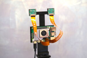
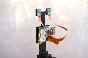
Last year I spent a lot of time on 3d-reconstructions, using the open-source program Meshroom. Semi-Global Matching (SGM)1 is a core component of the 3d-reconstruction process used in Meshroom and it’s also implemented in OpenCV for use in Stereo Vision. So to get some hands-on experience with SGM and Stereo Vision I bought a couple of RPi Camera Modules v3 and I 3d-printed a simple mount to hold them.
In this post I’ll first describe my setup, then we talk about the process of generating disparity maps and point clouds from stereo cameras and finally I’ll show an example.
Setup
Even though I’m using the Raspberry Pi 5 to take pictures, most of the stereo computation and visualization is done on my laptop. The RPi would be powerful enough to do the computations but my laptop is faster and the coding environment is already set up. So using the laptop is more convenient. To get the pictures captured by the RPi, I access them via WiFi on a Samba share that I’ve set up on the RPi.
Capturing Images
To capture images I ssh into the RPi and run a Python script. That script captures images from the two cameras as simultaneously as possible. Unfortunately, the RPi Camera Module v3 doesn’t provide a way to link the shutters of the two cameras so we can’t be certain that the image are taken at exactly the same moment2. I’m not worrying about that in this test because I’m looking at stationary scenes where nothing moves around. Still, I want to be able to use the code in more dynamic situations as well so I’m using the following lines of picamera2 code:
request0 = cam0.capture_request(wait=False)
request1 = cam1.capture_request(wait=False)

request0 = request0.get_result(timeout=5000)
request1 = request1.get_result(timeout=5000)
The method capture_request runs asynchronously, it doesn’t block the main thread, so the two cameras are told to take images without much delay between them.
To my knowledge, the cameras that I’m using here constantly stream images to the RPi. When we capture an image then the latest image in the buffer is copied, so capturing an image is very fast and the results should be available (almost) immediately.
There is a downside to not using the RPi directly: Without X-forwarding3 I can’t get a preview of what the cameras see. That’s a bit inconvenient but not a major issue for this test4.
Camera Calibration
Before we can do any sort of stereo vision we need to calibrate our cameras. First we do the regular camera calibration to get the camera matrix (focal length, principal point, image skew) and distortion coefficients. I’ve already made a couple of detailed videos about this topic here and here, so I won’t go into details in this post.
Then we can do the stereo calculation. The point of this step is to find the relative position of the two cameras. So we want to find the matrix R and the vector T that give us the relative rotation and translation of the first camera with respect to the second camera5. OpenCV provides the method:
res = cv.stereoCalibrate(
    objectPoints, imagePoints0, imagePoints1,
    cameraMatrix0, distortionCoefficients0,
    cameraMatrix1, distortionCoefficients1,
    imgSize, flags=cv.CALIB_FIX_INTRINSIC
)

retval, _, _, _, _, R, T, E, F = res
objectPoints refers to the world coordinates of our calibration target and imagePoints[i] refers to the coordinates of the object points on image i. I already have this data from the previous calibration step because I’m using the same images for the stereo calibration as I used for the two individual mono calibrations6.
The return value retval represents the total reprojection error of all points in all views of the cameras. This should be very small (0.27 in my case). E is the essential camera matrix and F is the fundamental matrix (which we won’t actually use here).
Rectification
At this point we’re able to undistort the images from our two cameras and we know the relative positions of the two cameras. So theoretically we could already run Semi-Global Matching.
Semi-Global Matching (or any other matching algorithm) searches for the best pixel matches over epipolar lines7. But right now the epipolar lines are not horizontal but they can be at any angle in the image. So searching over them is a bit tricky. This is where rectification comes in. The rectification step transforms the image so that all epipolar lines are horizontally aligned on our images. So when we run the SGM algorithm then we only need to search through pixels in the same row (which allows for a simpler implementation of the algorithm).
In OpenCV we can use the function:
res = cv.stereoRectify(
        cameraMatrix0, distortionCoefficients0,
        cameraMatrix1, distortionCoefficients1,
        imgSize, R, T, flags=cv.CALIB_ZERO_DISPARITY)

R0, R1, P0, P1, Q, ROI0, ROI1 = res
R0/R1 transform camera coordinates such that all epipolar lines end up being horizontally aligned (when projected onto the image). P0/P1 project these rectified points onto image coordinates (they represent an adjusted camera matrix). ROI0/ROI1 are the regions of interest, i.e. the largest rectangle in the resulting image that only contains valid data. Q is a matrix that allows us to convert the disparity map that we’ll compute soon back to 3d-coordinates (we’ll use that later).
Applying all Transformations
Before we run the matching algorithm we need to apply all of the transformations that we’ve talked about to the left and right images of our stereo setup. In OpenCV we can prepare a set of maps that specify how pixels are mapped between the original distorted, unrectified image and the undistorted, rectified image that we’ll use in the SGM algorithm8.
map0x, map0y = cv.initUndistortRectifyMap(
    cameraMatrix0, distortionCoefficients0,
    R0, P0, imgSize, cv.CV_32FC1)
This map only has to be created once and it can then be applied efficiently to any image that you want to correct. We apply it with the remap command:
img0_adj = cv.remap(img0, map0x, map0y, cv.INTER_LANCZOS4)Our maps don’t map to integral pixel values but rather to fractions of pixels. So to find the value at integral pixel coordinates we need to interpolate between all pixels that map to the vicinity of the target pixel. The last argument to cv.remap specifies the interpolation algorithm to use.
Semi-Global Matching
We’ve got rectified images where all epipolar lines are horizontal. Now we can run the matching algorithm. Our objective is to find the disparity for each pixel. That’s the horizontal distance between the pixel in the right image and the corresponding pixel in the left image. Objects that are closer to the cameras have a larger disparity than objects that are further away. So the disparity allows us to judge the relative distance of objects to our stereo cameras.
Let’s assume we’re looking for a match for pixel (x1, y1) in image 1, so in the right image. The possible candidates in image 0 are all pixels whose y-coordinate is y1 and whose x-coordinate is at least x1. At least because on the left image the matching pixel must be further on the right (check out the example images below if that sounds counterintuitive). We can limit the search interval by only looking at D pixels on the right of x1: {(x, y1) | x >= x1 and x < x1 + D}, which will work well as long as the maximum disparity is less than D.
Now we know where to look for matches, but how can we evaluate if two pixels match? A simple approach would be to directly compare the pixel (x1, y1) with each pixel in the search interval. We have to choose a metric for the comparison. For example, we could use something simple like the absolute difference of the pixel intensities, or something more complicated like a mutual information criterion.
Regardless of the criterion that we choose, this simple approach considers the match of pixel (x1, y1) in isolation of its neighbors. But that can be a problem. For example, there may be repeating patterns so (x1, y1) may match well with multiple pixels. Neighboring pixels in image 1 should match with pixels that are close to each other in image 0. So it would make sense to pick the matching pixel that’s closest to the match of the neighbors of (x1, y1), but that may not happen with a simple criterion like the one above. Noise could also affect the pixel values so we might get inaccurate matches even without repeating patterns.
To make sure that pixels that are close to each other in image 1 are also close to each other in image 0 we can add a second term to our criterion. This regularization term will depend on the distance between the matches of pixel (x1, y1) and the matches of its neighbors. Said differently, the regularization term depends on the disparity of adjacent pixels. In OpenCV this regularization term has value 0 if the disparity of neighboring pixels is 0, P1 if they differ by 1 and P2 if they differ by more than 1.
Ok, our cost function now has two components. The cost of the direct pixel matching and the cost of the regularization term related to the pixel’s neighbors. We can set the importance of the regularization term by adjusting the parameters P1 and P2.
So after carefully choosing P1 and P2 we should be able to get relatively consistent matches along a line of the image. But we’re not guaranteed to get consistent matches across lines. The matches of pixels in row 2 may not be very consistent with the matches of row 1. We could try to do this optimization globally, over the entire image, but that would be very expensive and it’s not certain that there would be a clear solution.
So instead, in Semi-Global Matching we consider the regularization term across neighbors in different directions. For example, we can look at the neighbors above and below in addition to the neighbors to the left and right of a pixel.
The version of SGM that’s implemented in OpenCV is a little different to the one in Hirschmüller’s paper, it’s initialized like this:
stereo = cv.StereoSGBM_create(
             minDisparity=0,
             numDisparities = 16,
             blockSize = 3,
             P1 = 0,
             P2 = 0,
             disp12MaxDiff = 0,
             uniquenessRatio = 0,
             speckleWindowSize = 0,
             speckleRange = 0,
             mode = cv.STEREO_SGBM_MODE_SGBM
)
The first argument minDisparity is the minimum x-distance between a pixel and it’s match (usually 0). numDisparities refers to the D we mentioned above, so to the maximum number of pixels that we look at along an epipolar line.
The method doesn’t actually match individual pixels but blocks of pixels, the argument blockSize determines the side length of such a block. P1 and P2 refer to the values of the regularization term. The argument mode determines how many directions the algorithm should consider. The default value shown here considers 5 directions but you can also choose more expensive and more accurate modes that use more directions. For the other parameters have a look at OpenCV’s documentation.
To compute the disparity map for two rectified stereo images we run this command:
disparity = stereo.compute(img0, img1).astype(np.float32) / 16.0The division by 16 is just a scaling factor.
Example
Let’s look at an example. I used my setup to capture two images. After distortion correction and rectification they look like this:

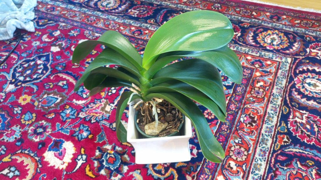
The camera on the left sees the flower further on the right, the camera on the right sees the flower further on the left. Now we need to decide upon good parameters for our Semi-Global Matching function. A priori it’s not so clear which parameters will give good results. The values
P1 = 8 * num_channels * 5**2
P2 = 32 * num_channels * 5**2
have been suggested as good starting points9 but we may have to adjust them for our specific example. To be able to play around with the parameters I wrote a little interactive matplotlib gui.
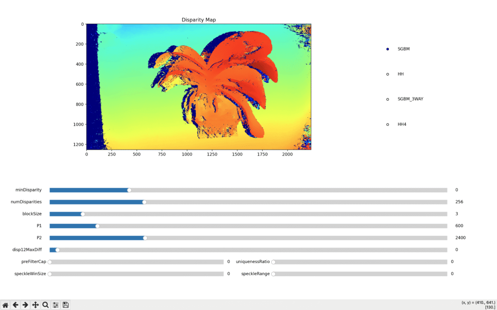
The image on the top shows the disparity map given the default settings. These default values usually work quite well. Although we may have to adjust them a little. Increasing uniquenessRatio helps to remove noisy matches10. Increasing P1 and P2 leads to a smoother disparity map (which isn’t always better). Speckle noise refers to areas with huge jumps in disparity. That can happen, for example, at the boundary of objects but it can also be introduced by noise in the image. To remove this noise a filter with parameters speckleWindowSize and speckleRange can be applied in post processing11.
A disparity map gives us relative distances but the units are related to pixel offsets. That’s not an issue for applications where only relative distances matter. But in some situations we’d rather have the distances in meters. So once we’re happy with our disparity map we can use it to compute the 3d-coordinates that correspond to the pixels on our disparity map. We use the matrix Q that we got in stereoRectify:
points = cv.reprojectImageTo3D(disparity, Q)I’ve plotted them with Open3D which looks like this:
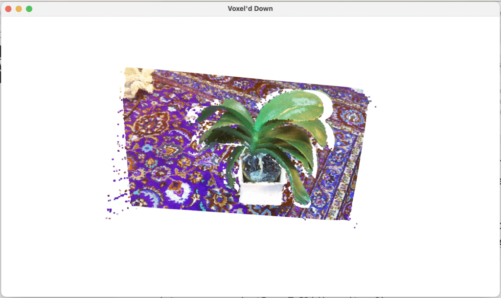
And after a little bit of outlier removal we get something like shown in the video below. A better camera/lens and more parameter tuning should result in a higher quality point cloud but I think the result is quite acceptable considering that I’m using two 25 EUR cameras.
Footnotes:
- Semi-Global Matching is not the only method that can be used to match pixels from two images. It is, however, a very common method because it’s both accurate and fast. ↩︎
- Other RPi cameras can do that. For example the Raspberry Pi High Quality Camera and the Raspberry Pi Global Shutter Camera allow you to either use an external trigger (such as a GPIO pin) or you can connect them in a master-slave setup using XVS (Vertical Sync Output). ↩︎
- I use Wayland on my laptop. You can apparently set up the equivalent to X-forwarding on Wayland but I haven’t yet had a chance to do that. ↩︎
- I initially ran the capture script on the RPi directly, with a screen connected to it. But the lower resolution preview of the two cameras resulted in a cropped image, even though I did set the correct aspect ratio in the preview configuration. So the preview wasn’t very useful because it would only provide a rough estimate of the picture. I didn’t use it in the end because I can also get a rough estimate of the picture by looking (with my own eyes) where the cameras are pointing. ↩︎
- Or equivalently, it tells us how points in the coordinate system of camera 1 get mapped to the coordinate system of camera 2. ↩︎
- Let me be more specific. When taking the calibration pictures I moved the camera around and at each position my script took a photo with each camera. At some positions one of the cameras didn’t capture the entire calibration target. For example, if the right camera captures the target at its left edge then the left camera won’t be able to capture the entire target. Those images are excluded from the stereo calibration. Only images where both cameras capture the full target are included. ↩︎
- Check out https://en.wikipedia.org/wiki/Epipolar_geometry if you’re not familiar with epipolar geometry. ↩︎
- To be able to compute the transforms efficiently the maps tell us how to go from the undistorted/rectified image to the distorted/unrectified image. So map0x[y, x] returns the x-coordinate in the distorted image that corresponds to the x/y coordinates in the undistorted image. That may sound counter-intuitive because our input are distorted images, nevertheless the computation is faster this way. ↩︎
- ↩︎
- It refers to how much better the cost function value of the best match must be compared to the cost function value of the next best match. If the actual ratio is below uniquenessRatio then the candidate match is considered invalid and no match is found. ↩︎
- This stackoverflow post describes quite nicely how the speckle filter works. ↩︎
Leave a Reply